

Mann-Kendall Trend Test & Theil-Sen Slope Calculator
Free Mann-Kendall trend test calculator with Theil-Sen slope estimator. Compute S statistic, tie-corrected Var(S), continuity-corrected Z, p-value, and Kendall's tau in your browser.
Open toolLocate structural mean shifts and regime boundaries in any numeric time series: run exact `O(N^2)` dynamic programming (Optimal Partitioning / PELT objective with BIC, AIC, or custom penalties) alongside cumulative sum (`CUSUM`) peak detection.
Enter the inputs, then select Detect Change Points.
Result will appear here
Instead of greedy binary splitting, this tool solves the exact global penalized least-squares objective across all valid segmentations.
Penalized Cost: min_{m, tau_1..tau_m} [ sum_{k=1}^{m+1} SSE(y_{tau_{k-1}+1 : tau_k}) + m * beta ], where SSE(y_{a:b}) = sum_{t=a}^b (y_t - mean(y_{a:b}))^2 and robust noise variance sigma^2 = median((Delta y_t)^2 / 2) / 0.454936; CUSUM Statistic: S_t = sum_{i=1}^t (y_i - mean(y)).
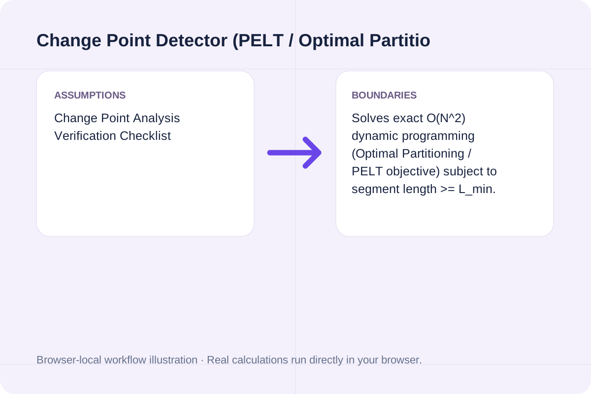
Solves exact O(N^2) dynamic programming (Optimal Partitioning / PELT objective) subject to segment length >= L_min. Robust diff-based variance estimation prevents large true mean shifts from inflating sigma^2.
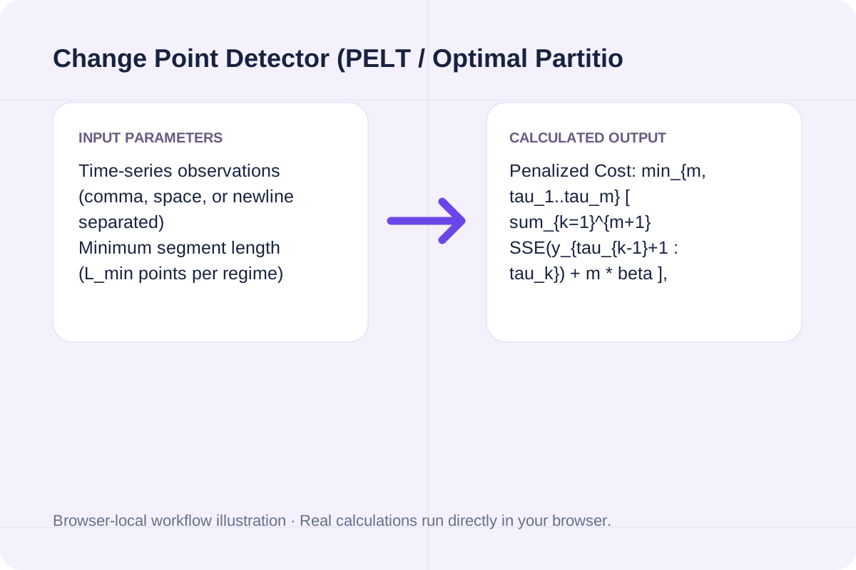
Comparison of penalty criteria (`BIC`, `AIC`, `Manual`) and exact output on the default 12-point step-shift series (`10.05` -> `24.95` at Index `#7`).
| Component / Metric | Mathematical Definition | Default 12-Point Series Result | Practical Guidance |
|---|---|---|---|
| **Detected Change Point (`tau_1`)** | First index of the new regime (`y_{tau_1}`) | **Index `#7`** (`value = 24.80`, after `#6 = 10.30`) | Splits `N = 12` into `[#1..#6]` and `[#7..#12]` |
| **Regime Means & Step Shift** | `mu_1 = mean(y_{1:6})`, `mu_2 = mean(y_{7:12})` | `mu_1 = 10.0500`, `mu_2 = 24.9500` (`Shift = +14.9000`) | Exact piecewise constant step model |
| **Total vs. Residual Sum of Squares** | `TSS = sum(y_i - y_bar)^2`, `RSS = sum(SSE_k)` | `TSS = 666.3800` -> `RSS = 0.3500` (`R^2 = 99.95%`) | 99.95% of total variance is explained by the 1 shift |
| **BIC Penalty (`beta_BIC`)** | `2 * sigma_hat^2 * ln(N) * multiplier` | Prevents false splits inside noisy plateaus | Recommended default for unknown breakpoint count `m` |
| **Peak CUSUM Index** | `argmax_t |sum_{i=1}^t (y_i - y_bar)|` | Peaks at boundary `#6 / #7` (`|CUSUM| = 44.7000`) | Confirms primary shift location independently |
Enter the values for your scenario, verify the units, and run the calculation.
Start by entering the required fields in the Change Point Detector (PELT / Optimal Partitioning & CUSUM) form above.
Match each value to the unit or format shown next to the input box before running the calculation.
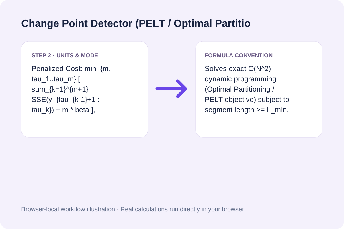
Select Detect Change Points, inspect the primary metric and breakdown cards, then use Copy result or Download result.txt.
Compare baseline and alternative runs for Change Point Detector (PELT / Optimal Partitioning & CUSUM) before exporting the result.
Detect multiple change points and regime shifts in a numeric time series using exact O(N^2) dynamic programming (BIC, AIC, or custom penalty) and CUSUM statistics.
Penalized Cost: min_{m, tau_1..tau_m} [ sum_{k=1}^{m+1} SSE(y_{tau_{k-1}+1 : tau_k}) + m * beta ], where SSE(y_{a:b}) = sum_{t=a}^b (y_t - mean(y_{a:b}))^2 and robust noise variance sigma^2 = median((Delta y_t)^2 / 2) / 0.454936; CUSUM Statistic: S_t = sum_{i=1}^t (y_i - mean(y)).
Solves exact O(N^2) dynamic programming (Optimal Partitioning / PELT objective) subject to segment length >= L_min. Robust diff-based variance estimation prevents large true mean shifts from inflating sigma^2.
Review the calculated output alongside your entered parameters and unit conventions.
Solves exact O(N^2) dynamic programming (Optimal Partitioning / PELT objective) subject to segment length >= L_min. Robust diff-based variance estimation prevents large true mean shifts from inflating sigma^2.
Check these three items before acting on a detected breakpoint.
Penalized Cost: min_{m, tau_1..tau_m} [ sum_{k=1}^{m+1} SSE(y_{tau_{k-1}+1 : tau_k}) + m * beta ], where SSE(y_{a:b}) = sum_{t=a}^b (y_t - mean(y_{a:b}))^2 and robust noise variance sigma^2 = median((Delta y_t)^2 / 2) / 0.454936; CUSUM Statistic: S_t = sum_{i=1}^t (y_i - mean(y)). Solves exact O(N^2) dynamic programming (Optimal Partitioning / PELT objective) subject to segment length >= L_min. Robust diff-based variance estimation prevents large true mean shifts from inflating sigma^2.
Free Mann-Kendall trend test calculator with Theil-Sen slope estimator. Compute S statistic, tie-corrected Var(S), continuity-corrected Z, p-value, and Kendall's tau in your browser.
Open tool
Calculate Dynamic Time Warping (DTW) distance and optimal alignment path between two time series in your browser. Supports absolute, squared, and root-squared costs plus Sakoe-Chiba window band.
Open tool
Calculate bottleneck cycle time, Takt time margin, hourly and shift throughput, line balance efficiency, flow efficiency, and Little's Law WIP from workstation times.
Open toolChoose another tool for your next calculation, conversion, or text task.

Calculate Cohen's d, Hedges' g, Glass's delta, correlation r, 95% confidence interval, and Cohen's U3 / CLES from group means, standard deviations, and sample sizes.
Open tool
Free Kaplan-Meier survival calculator. Compute product-limit survival S(t), Greenwood variance, log-log or linear confidence intervals, median survival time, and risk-set tables in your browser.
Open tool
Calculate the Mantel-Cox log-rank test statistic (chi-square, df = 1), p-value, observed vs. expected events, hypergeometric variance, and hazard ratio from censored survival data.
Open tool
Calculate sample size for comparing two independent means, testing a single mean, or estimating a mean within a target margin of error. Includes Z-approximation, ceiling rounding, and allocation ratio k = n2/n1.
Open toolAnswers about using Change Point Detector (PELT / Optimal Partitioning & CUSUM) and understanding its results.
Adding a breakpoint always reduces residual sum of squares (RSS), so an unpenalized fit would split the series into as many tiny segments as allowed. Optimal Partitioning minimizes Total Cost = sum(SSE_k) + m * beta, adding a breakpoint only when the reduction in SSE exceeds the penalty beta.
If a time series jumps from 10 to 25, the global sample variance is dominated by the +15 step jump rather than within-regime noise. Estimating sigma^2 from consecutive differences (using the robust median squared difference estimator divided by 2 * 0.454936, the chi-square median for df = 1) isolates true within-segment noise so BIC and AIC penalties scale accurately.
Cumulative Sum (CUSUM) computes S_t = sum_{i=1}^t (y_i - mean(y)) and finds the single index t* where |S_t| is maximized, which is ideal for spotting the primary single shift in quality control charts. The dynamic programming solver simultaneously finds 0, 1, or multiple change points (tau_1, tau_2, ...) across the entire series.
Set L_min to the shortest duration that represents a meaningful regime rather than a transient spike. Setting L_min >= 3 prevents a single isolated outlier from being flagged as its own two-breakpoint regime.
Choose another tool for your next calculation, conversion, or text task.