

Change Point Detector (PELT / Optimal Partitioning & CUSUM)
Detect multiple change points and regime shifts in a numeric time series using exact O(N^2) dynamic programming (BIC, AIC, or custom penalty) and CUSUM statistics.
Open toolCompute the exact **Dynamic Time Warping (DTW)** distance, normalized per-step cost, optimal alignment path `(i, j)`, and accumulated dynamic-programming cost matrix `D(i, j)` between two numeric sequences of equal or unequal length.
Enter the inputs, then select Calculate DTW Distance & Path.
Result will appear here
Paste two numeric series of any length (up to 150 observations each) to run the exact O(n×m) dynamic programming solver.
D(i, j) = c(x_i, y_j) + min( D(i−1, j), D(i, j−1), D(i−1, j−1) ) subject to |i − j| ≤ w (when w > 0); Normalized Cost = D(n, m) / K, where K is the number of aligned steps in the optimal warping path.
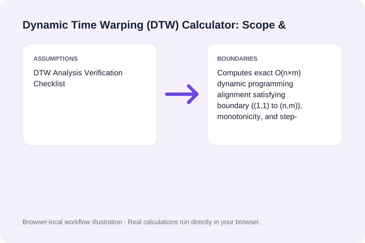
Computes exact O(n×m) dynamic programming alignment satisfying boundary ((1,1) to (n,m)), monotonicity, and step-continuity constraints, and compares DTW against lock-step Euclidean/Manhattan distance.
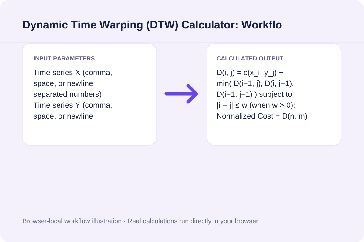
Summary of local cost options, dynamic programming recurrence rules, and output metrics computed on this page.
| Metric / Parameter | Mathematical Definition | Default Sample Value (`X` vs `Y`) | Practical Interpretation |
|---|---|---|---|
| Local Cost `c(x_i, y_j)` | `|x_i − y_j|` or `(x_i − y_j)²` | `|x_i − y_j|` (Absolute) | Point-to-point discrepancy before cumulative DP warping |
| DP Recurrence `D(i, j)` | `c(x_i,y_j) + min(D(i−1,j−1), D(i−1,j), D(i,j−1))` | **`DTW = 1.00`** | Minimum cumulative cost to align prefixes `X[1..i]` and `Y[1..j]` |
| Normalized Path Cost | `DTW / K` (`K` = warping path length) | **`0.1250 / step`** (`K = 8`) | Average alignment error per step along the optimal path |
| Lock-Step Baseline | `∑ |x_i − y_i|` (when `n = m`) | `16.00` (vs. `1.00` DTW) | Shows how much phase-shift distortion DTW removes (`93.75%` lower) |
Enter the values for your scenario, verify the units, and run the calculation.
Start by entering the required fields in the Dynamic Time Warping (DTW) Calculator form above.
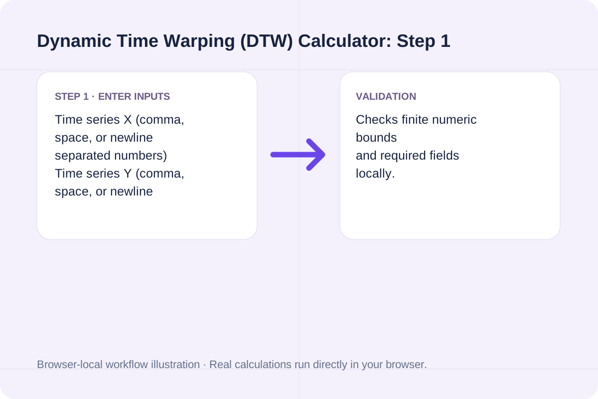
Match each value to the unit or format shown next to the input box before running the calculation.
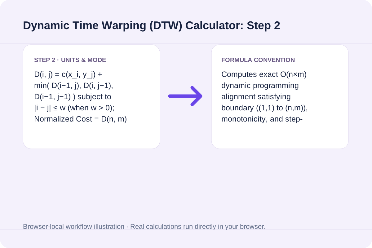
Select Calculate DTW Distance & Path, inspect the primary metric and breakdown cards, then use Copy result or Download result.txt.
Compare baseline and alternative runs for Dynamic Time Warping (DTW) Calculator before exporting the result.
Calculate Dynamic Time Warping (DTW) distance and optimal alignment path between two time series in your browser. Supports absolute, squared, and root-squared costs plus Sakoe-Chiba window band.
D(i, j) = c(x_i, y_j) + min( D(i−1, j), D(i, j−1), D(i−1, j−1) ) subject to |i − j| ≤ w (when w > 0); Normalized Cost = D(n, m) / K, where K is the number of aligned steps in the optimal warping path.
Computes exact O(n×m) dynamic programming alignment satisfying boundary ((1,1) to (n,m)), monotonicity, and step-continuity constraints, and compares DTW against lock-step Euclidean/Manhattan distance.
Review the calculated output alongside your entered parameters and unit conventions.
Computes exact O(n×m) dynamic programming alignment satisfying boundary ((1,1) to (n,m)), monotonicity, and step-continuity constraints, and compares DTW against lock-step Euclidean/Manhattan distance.
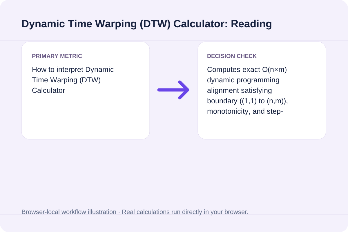
Check these three items when interpreting DTW distances.
D(i, j) = c(x_i, y_j) + min( D(i−1, j), D(i, j−1), D(i−1, j−1) ) subject to |i − j| ≤ w (when w > 0); Normalized Cost = D(n, m) / K, where K is the number of aligned steps in the optimal warping path. Computes exact O(n×m) dynamic programming alignment satisfying boundary ((1,1) to (n,m)), monotonicity, and step-continuity constraints, and compares DTW against lock-step Euclidean/Manhattan distance.
Detect multiple change points and regime shifts in a numeric time series using exact O(N^2) dynamic programming (BIC, AIC, or custom penalty) and CUSUM statistics.
Open tool
Free Kaplan-Meier survival calculator. Compute product-limit survival S(t), Greenwood variance, log-log or linear confidence intervals, median survival time, and risk-set tables in your browser.
Open tool
Calculate sample size for comparing two independent means, testing a single mean, or estimating a mean within a target margin of error. Includes Z-approximation, ceiling rounding, and allocation ratio k = n2/n1.
Open toolChoose another tool for your next calculation, conversion, or text task.

Calculate Cohen's d, Hedges' g, Glass's delta, correlation r, 95% confidence interval, and Cohen's U3 / CLES from group means, standard deviations, and sample sizes.
Open tool
Calculate the Mantel-Cox log-rank test statistic (chi-square, df = 1), p-value, observed vs. expected events, hypergeometric variance, and hazard ratio from censored survival data.
Open tool
Free Mann-Kendall trend test calculator with Theil-Sen slope estimator. Compute S statistic, tie-corrected Var(S), continuity-corrected Z, p-value, and Kendall's tau in your browser.
Open tool
Free sample size calculator for comparing two independent proportions (p1 vs. p2). Compute unadjusted and Fleiss continuity-corrected n1, n2, total N, and Cohen's h.
Open toolAnswers about using Dynamic Time Warping (DTW) Calculator and understanding its results.
Lock-step Euclidean or Manhattan distance compares index i of series X strictly against the same index i of series Y (and cannot compare series of unequal length). If two identical waveforms are shifted by even a single time step—such as X = [1, 3, 4, 9, 8, 2, 1] and Y = [1, 1, 3, 4, 9, 8, 2]—lock-step distance reports a large error (16.0), whereas DTW nonlinearly stretches the time axis and finds a near-zero alignment cost (1.0).
A standard DTW warping path W = [w_1, ..., w_K] must satisfy: (1) Boundary condition: start at w_1 = (1, 1) and end at w_K = (n, m); (2) Continuity: each step moves by at most 1 index in i and j, i.e., (i_k − i_{k−1}, j_k − j_{k−1}) ∈ {(1,0), (0,1), (1,1)}; and (3) Monotonicity: indices never move backward in time (i_k ≥ i_{k−1} and j_k ≥ j_{k−1}).
The Sakoe-Chiba band constrains the warping path so that index i in series X can only align with index j in series Y if |i − j| ≤ max(w, |n − m|). Setting a locality window prevents pathological warping (where a single point in X stretches across dozens of points in Y) and speeds up computation.
Raw DTW distance sums the local costs across all K steps of the warping path, so longer sequences naturally accumulate larger raw sums. Dividing the total DTW cost by the warping path length K yields the Normalized Path Cost per aligned step, allowing fair similarity comparisons across pairs of different lengths.
Choose another tool for your next calculation, conversion, or text task.