

Log-Rank Test Calculator (Mantel-Cox Survival Analysis)
Calculate the Mantel-Cox log-rank test statistic (chi-square, df = 1), p-value, observed vs. expected events, hypergeometric variance, and hazard ratio from censored survival data.
Open toolPaste right-censored time-to-event data (`time, status`) to compute the Kaplan-Meier product-limit survival curve `S(t)`, Greenwood standard error, 95% log-log confidence intervals, restricted mean survival time (RMST), and median survival time `t_50`.
Enter the inputs, then select Calculate Kaplan-Meier Curve.
Result will appear here
Introduced by Edward L. Kaplan and Paul Meier in 1958, the product-limit estimator calculates non-parametric survival probabilities from incomplete (right-censored) follow-up records without assuming an exponential or Weibull distribution.
S(t) = prod_{t_i <= t} ((n_i - d_i) / n_i); Greenwood SE = S(t) * sqrt(sum d_i / (n_i * (n_i - d_i))); RMST(tau) = sum S(t_{i-1}) * (t_i - t_{i-1}).
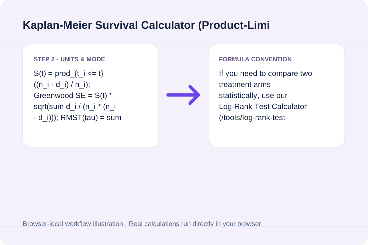
If you need to compare two treatment arms statistically, use our Log-Rank Test Calculator (/tools/log-rank-test-calculator) alongside this curve estimator.
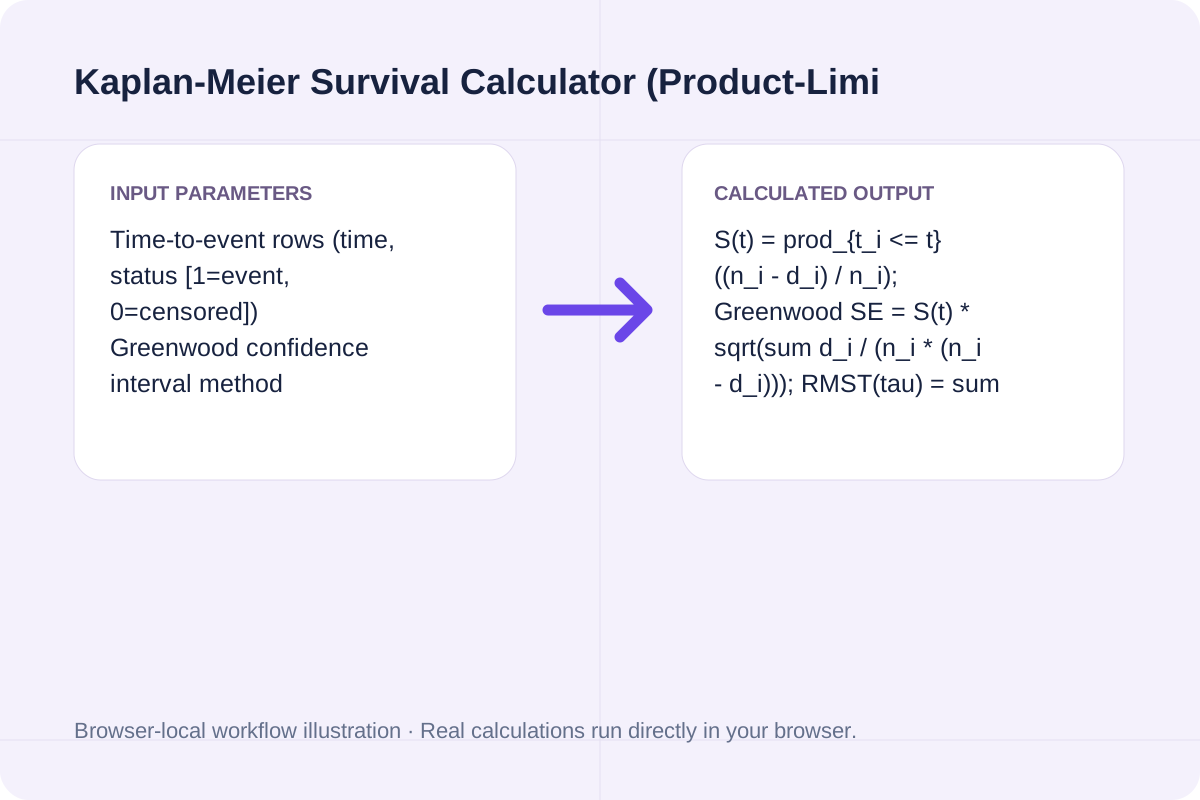
Core survival formulas, tie-breaking rules, and exact outputs for the default 10-subject clinical follow-up cohort.
| Biostatistics Metric | Exact Formula / Rule | Default Cohort Output (`N = 10`, `6` Events) | Clinical / Engineering Meaning |
|---|---|---|---|
| Product-Limit Survival `S(t)` | `prod_{t_i <= t} (1 - d_i / n_i)` | `S(12) = 0.5486` (`54.86%`) | Probability of surviving past landmark time `t* = 12` |
| Greenwood Standard Error `SE(S(t))` | `S(t) * sqrt(sum [d_i / (n_i * (n_i - d_i))])` | `SE(12) = 0.1724` at `t* = 12` | Sampling uncertainty of the step survival estimate |
| 95% Complementary Log-Log CI | `S(t)^{exp(+- 1.96 * sigma_u)}` | `[0.1950, 0.8065]` at `t* = 12` | Range-preserving confidence interval bounded in `(0, 1)` |
| Median Survival Time (`t_50`) | `min { t_i : S(t_i) <= 0.50 }` | `t_50 = 15` time units (`S(15) = 0.4114`) | Earliest timestamp where half the cohort has experienced the event |
| Restricted Mean Survival (RMST) | `integral_0^{t_max} S(u) du` | `14.36` time units (up to `t = 24`) | Area under the Kaplan-Meier staircase up to horizon `t_max` |
Generate a publication-ready survival table and landmark confidence intervals in seconds.
Paste one subject per row as 'time, status' where status = 1 indicates an observed event (death, relapse, component failure, churn) and status = 0 indicates a right-censored record.
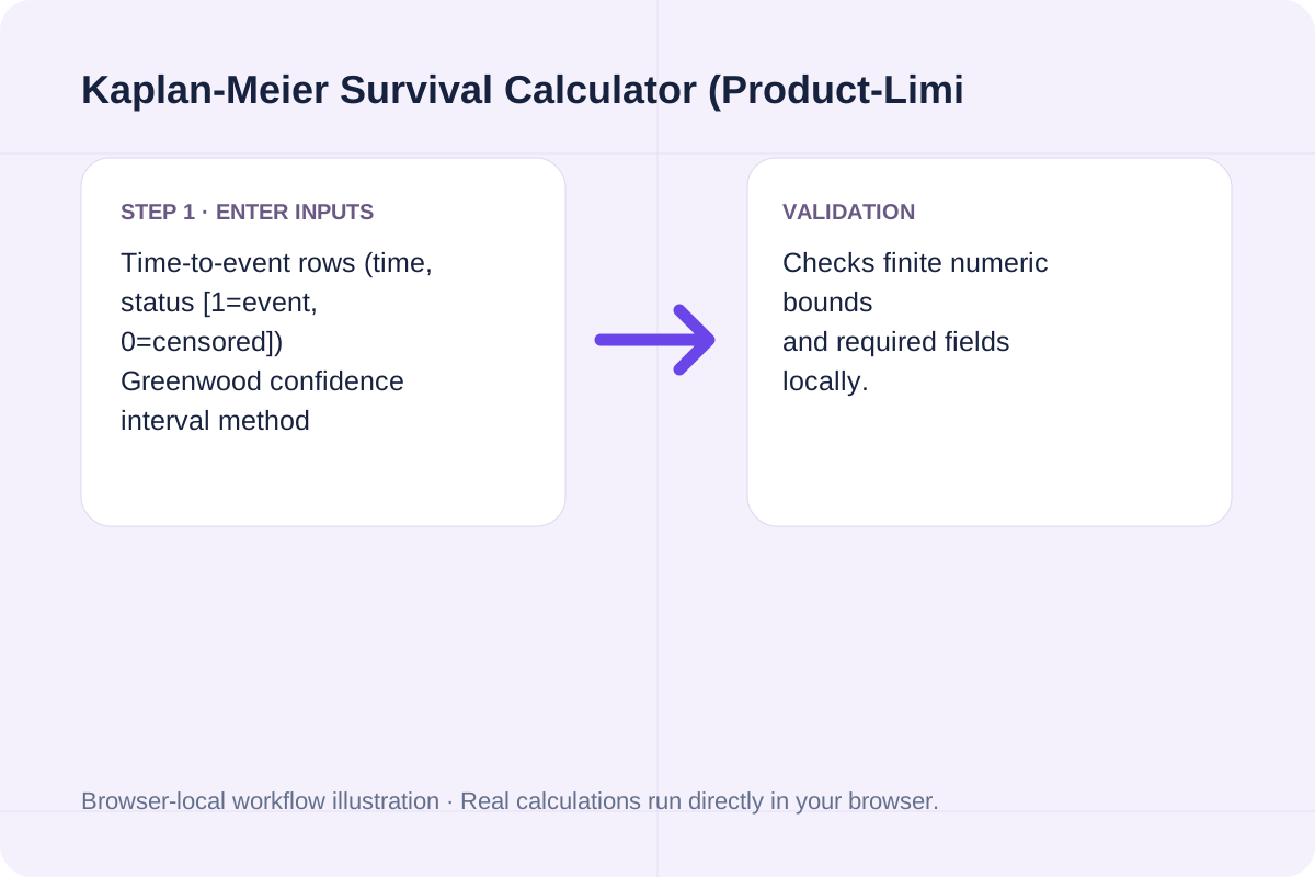
Choose between the complementary log-log confidence interval (default in R survfit and SAS) or plain linear Greenwood bounds, and specify a landmark time t* to query.
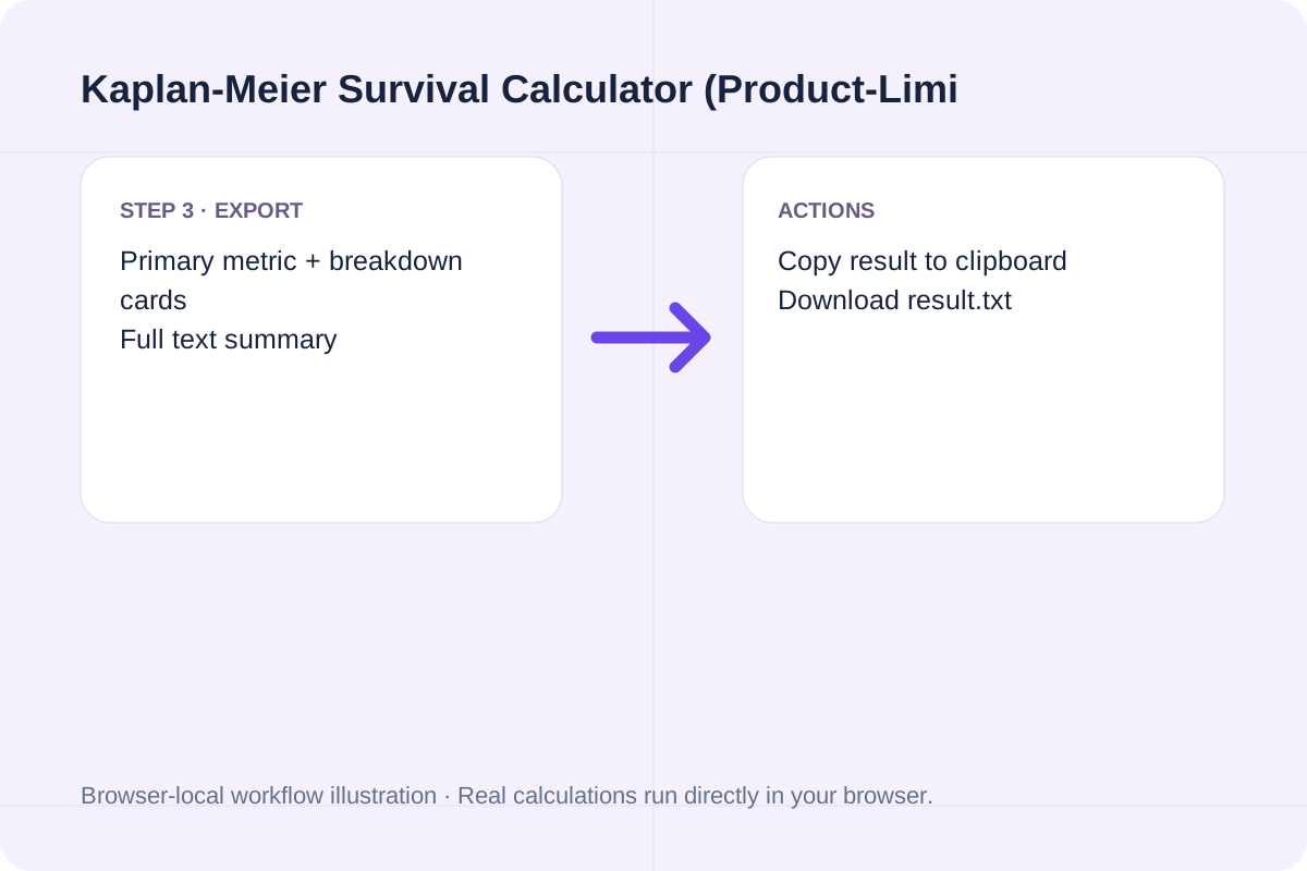
Review the landmark survival S(t*), median survival time t_50, restricted mean survival time (RMST), and export the complete step table showing n_i, d_i, c_i, S(t_i), SE, and CI.
Verify the product-limit steps and Greenwood variance on real biostatistics scenarios.
Free Kaplan-Meier survival calculator. Compute product-limit survival S(t), Greenwood variance, log-log or linear confidence intervals, median survival time, and risk-set tables in your browser.
S(t) = prod_{t_i <= t} ((n_i - d_i) / n_i); Greenwood SE = S(t) * sqrt(sum d_i / (n_i * (n_i - d_i))); RMST(tau) = sum S(t_{i-1}) * (t_i - t_{i-1}).
If you need to compare two treatment arms statistically, use our Log-Rank Test Calculator (/tools/log-rank-test-calculator) alongside this curve estimator.
Combine point survival estimates with the at-risk sample size n_i when reading the tail of a survival curve.
First, watch the risk set n_i in the final columns of follow-up. When heavy censoring reduces n_i below 5 subjects, a single late event causes a dramatic vertical drop in S(t) and widens the Greenwood 95% confidence interval.
Second, when fewer than 50% of subjects experience the event before the study ends, the median survival time t_50 is not reached; in that case, report the Restricted Mean Survival Time (RMST) up to the study horizon tau and the landmark survival probability S(tau).
Ensure your time-to-event dataset satisfies these three non-parametric assumptions.
1. Independent (Non-Informative) Censoring: Right-censored subjects at time t must have the same future hazard rate as subjects who remain under observation at time t.
2. Exact Tie-Handling Convention: When an event (1) and a censoring (0) share the exact same timestamp t, the event is evaluated first (so the censored subject contributes to the risk set n_i at time t) before being removed for t > t_i.
Calculate the Mantel-Cox log-rank test statistic (chi-square, df = 1), p-value, observed vs. expected events, hypergeometric variance, and hazard ratio from censored survival data.
Open tool
Calculate Cohen's d, Hedges' g, Glass's delta, correlation r, 95% confidence interval, and Cohen's U3 / CLES from group means, standard deviations, and sample sizes.
Open tool
Calculate Dynamic Time Warping (DTW) distance and optimal alignment path between two time series in your browser. Supports absolute, squared, and root-squared costs plus Sakoe-Chiba window band.
Open toolChoose another tool for your next calculation, conversion, or text task.

Free Mann-Kendall trend test calculator with Theil-Sen slope estimator. Compute S statistic, tie-corrected Var(S), continuity-corrected Z, p-value, and Kendall's tau in your browser.
Open tool
Detect multiple change points and regime shifts in a numeric time series using exact O(N^2) dynamic programming (BIC, AIC, or custom penalty) and CUSUM statistics.
Open tool
Free sample size calculator for comparing two independent proportions (p1 vs. p2). Compute unadjusted and Fleiss continuity-corrected n1, n2, total N, and Cohen's h.
Open tool
Calculate sample size for comparing two independent means, testing a single mean, or estimating a mean within a target margin of error. Includes Z-approximation, ceiling rounding, and allocation ratio k = n2/n1.
Open toolAnswers about using Kaplan-Meier Survival Calculator (Product-Limit & Greenwood CI) and understanding its results.
Subjects who are right-censored (status = 0, such as patients still alive at study close or lost to follow-up) remain in the at-risk denominator n_i for every event time up to and including their censoring timestamp. Immediately after their censoring time, they are removed from n_i without reducing the survival probability S(t).
Plain linear bounds S(t) +- z * SE(S(t)) can drop below 0.0 or exceed 1.0 near the start or tail of follow-up. Transforming survival onto the complementary log-log scale u = ln(-ln(S(t))) and exponentiating back ensures both lower and upper confidence bounds always remain strictly within (0, 1).
Median survival time t_50 is the smallest event time t_i at which the estimated survival probability S(t_i) falls to 0.50 (50%) or below. If S(t) remains strictly above 0.50 at the final observation, median survival is reported as 'Not reached' (> max follow-up).
Use this Kaplan-Meier Calculator to estimate the survival curve S(t), Greenwood confidence bands, and median survival for a single cohort. To test whether two cohorts' survival curves differ significantly, pass both groups into our Log-Rank Test Calculator (/tools/log-rank-test-calculator).
Choose another tool for your next calculation, conversion, or text task.