

Lawn Mowing Time Calculator (Deck Width, Overlap, Speed & Acres/Hr)
Calculate how long it takes to mow any lawn size by deck width, mowing speed, pass overlap, and turn/obstacle field efficiency.
Open toolPinpoint your slowest workstation and quantify flow losses: calculate bottleneck cycle time (`CT_max`), Takt time margin, hourly and shift throughput, line balance efficiency (`LBE`), flow efficiency, and Little's Law equilibrium WIP.
Enter the inputs, then select Analyze Cycle Time & Flow.
Result will appear here
A multi-stage workflow is constrained by its bottleneck pace (`CT_max`) and its total accumulated queue delay (`T_wait`).
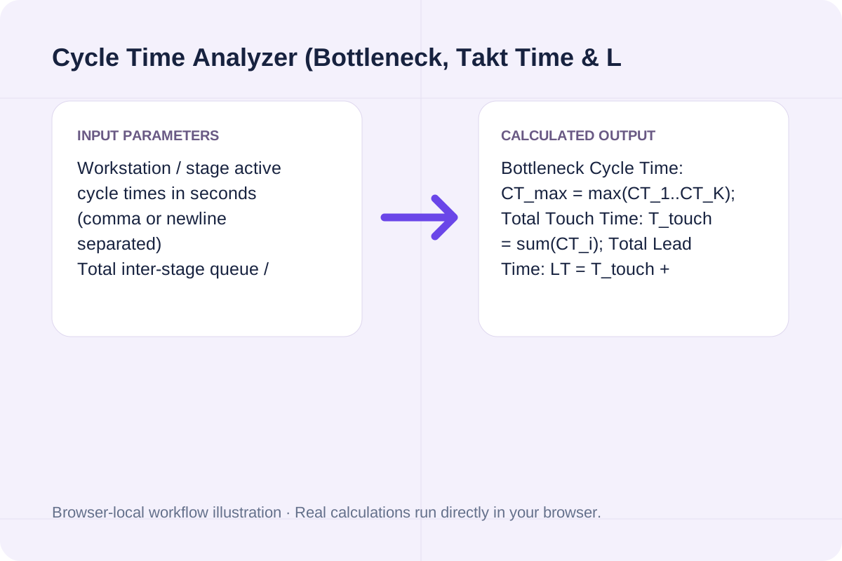
Bottleneck Cycle Time: CT_max = max(CT_1..CT_K); Total Touch Time: T_touch = sum(CT_i); Total Lead Time: LT = T_touch + T_wait; Takt Time = (Available_Min * 60) / Demand; Hourly Capacity = 3600 / CT_max; Line Balance Efficiency (LBE) = T_touch / (K * CT_max) * 100%; Flow Efficiency = (T_touch / LT) * 100%; Little's Law WIP = LT / CT_max.
In a serial production line without parallel station duplication, total line throughput is strictly bounded by the slowest station (CT_max). Little's Law (WIP = Throughput * Lead Time) represents steady-state average work-in-progress.
Core lean manufacturing formulas and exact benchmark metrics for the default 5-station line (`18s, 24s, 42s, 30s, 21s`, `265s` queue wait, `450 min` shift, `600` units demand).
| Flow Metric | Exact Formula | Default 5-Station Output | Operational Benchmark / Rule |
|---|---|---|---|
| **Bottleneck Cycle Time (`CT_max`)** | `max(CT_1, CT_2, ..., CT_K)` | `42.00 s/unit` (Station #3) | Governs pace of the entire serial line (`85.71 units/hr`) |
| **Customer Takt Time** | `(Available_Min * 60) / Shift_Demand` | `45.00 s/unit` (`27,000s / 600`) | `CT_max <= Takt` required (`+3.00s` safety margin) |
| **Shift Capacity vs. Demand** | `floor((Available_Min * 60) / CT_max)` | `642 units/shift` vs. `600` target | `+42 units` (`+7.05%`) buffer per 450-minute shift |
| **Line Balance Efficiency (`LBE`)** | `sum(CT_i) / (K * CT_max) * 100%` | `64.29%` (`135s / 210s`) | World-class assembly lines target `LBE >= 85%` |
| **Flow Efficiency & Little's Law WIP** | `T_touch / (T_touch + T_wait)`, `WIP = LT / CT_max` | `33.75%` flow (`135s / 400s`), `WIP = 9.52 units` | Reducing queue wait lowers WIP and lead time proportionally |
Enter the values for your scenario, verify the units, and run the calculation.
Start by entering the required fields in the Cycle Time Analyzer (Bottleneck, Takt Time & Little's Law WIP) form above.
Match each value to the unit or format shown next to the input box before running the calculation.
Select Analyze Cycle Time & Flow, inspect the primary metric and breakdown cards, then use Copy result or Download result.txt.
Compare baseline and alternative runs for Cycle Time Analyzer (Bottleneck, Takt Time & Little's Law WIP) before exporting the result.
Calculate bottleneck cycle time, Takt time margin, hourly and shift throughput, line balance efficiency, flow efficiency, and Little's Law WIP from workstation times.
Bottleneck Cycle Time: CT_max = max(CT_1..CT_K); Total Touch Time: T_touch = sum(CT_i); Total Lead Time: LT = T_touch + T_wait; Takt Time = (Available_Min * 60) / Demand; Hourly Capacity = 3600 / CT_max; Line Balance Efficiency (LBE) = T_touch / (K * CT_max) * 100%; Flow Efficiency = (T_touch / LT) * 100%; Little's Law WIP = LT / CT_max.
In a serial production line without parallel station duplication, total line throughput is strictly bounded by the slowest station (CT_max). Little's Law (WIP = Throughput * Lead Time) represents steady-state average work-in-progress.
Review the calculated output alongside your entered parameters and unit conventions.
In a serial production line without parallel station duplication, total line throughput is strictly bounded by the slowest station (CT_max). Little's Law (WIP = Throughput * Lead Time) represents steady-state average work-in-progress.
Avoid these three common measurement errors during time studies.
Bottleneck Cycle Time: CT_max = max(CT_1..CT_K); Total Touch Time: T_touch = sum(CT_i); Total Lead Time: LT = T_touch + T_wait; Takt Time = (Available_Min * 60) / Demand; Hourly Capacity = 3600 / CT_max; Line Balance Efficiency (LBE) = T_touch / (K * CT_max) * 100%; Flow Efficiency = (T_touch / LT) * 100%; Little's Law WIP = LT / CT_max. In a serial production line without parallel station duplication, total line throughput is strictly bounded by the slowest station (CT_max). Little's Law (WIP = Throughput * Lead Time) represents steady-state average work-in-progress.
Calculate how long it takes to mow any lawn size by deck width, mowing speed, pass overlap, and turn/obstacle field efficiency.
Open tool
Calculate hiking time from trail distance, elevation gain, elevation loss, base flat pace, and terrain difficulty using Naismith's Rule, Langmuir descent adjustments, and Tobler's function.
Open tool
Determine reaction order (0th, 1st, or 2nd) from time-concentration data by linearizing [A], ln[A], and 1/[A] vs. time t, comparing R² and RMSE, and calculating rate constant k and half-life.
Open toolChoose another tool for your next calculation, conversion, or text task.

Calculate oligonucleotide primer melting temperature (Tm) using SantaLucia 1998 Nearest-Neighbor thermodynamics, Salt-Adjusted Marmur-Doty, and Wallace rules.
Open tool
Analyze warehouse fulfillment performance from order line data: compute unit fill rate, line fill rate, order fill rate, and backorder recovery with explicit gross vs. net denominators.
Open tool
Calculate room reverberation time (RT60) using Sabine (0.161 V / A) and Norris-Eyring formulas from room volume and surface absorption coefficients.
Open tool
Calculate CNC milling and turning Metal Removal Rate (MRR in cm³/min and in³/min), estimated spindle power (kW / HP), and chip load.
Open toolAnswers about using Cycle Time Analyzer (Bottleneck, Takt Time & Little's Law WIP) and understanding its results.
Cycle Time (CT) is the actual time required for a workstation (or the bottleneck station CT_max) to complete one unit. Takt Time is the customer demand pace (Available Net Production Seconds divided by Customer Demand Units). Lead Time (LT, or turnaround time) is the total elapsed time a single item takes from raw input to finished output, equal to Total Active Touch Time plus Total Queue Wait Time.
Line Balance Efficiency measures how evenly work is distributed across K sequential stations: LBE = (sum of all station cycle times) / (K * CT_max) * 100%. If 5 stations take 18s, 24s, 42s, 30s, and 21s (sum = 135s, bottleneck CT_max = 42s), LBE = 135 / (5 * 42) = 64.29%, meaning 35.71% of station capacity is lost to starvation or blocking waiting on Station #3.
Little's Law states that average Work-In-Progress equals Throughput multiplied by Lead Time (WIP = lambda * LT). Since steady-state line throughput is lambda = 1 / CT_max units per second, equilibrium WIP is simply LT / CT_max. With a 400-second lead time and a 42-second bottleneck cycle time, the line holds an average of 400 / 42 = 9.52 units in progress.
When CT_max > Takt Time, the line cannot meet shift demand without overtime. You can either split tasks from the bottleneck station onto adjacent under-utilized stations (line balancing), add a parallel workstation at the bottleneck (halving its effective cycle time), or apply SMED / process improvements to reduce active cycle seconds.
Choose another tool for your next calculation, conversion, or text task.