

Reaction Rate Calculator
Calculate average chemical reaction rate, reactant consumption rate, apparent rate constant k, and half-life from initial and final molarity and Δt.
Open toolEnter experimental time and molar concentration pairs (`t, [A]`) to simultaneously regress Zero-Order (`[A]` vs. `t`), First-Order (`ln[A]` vs. `t`), and Second-Order (`1/[A]` vs. `t`) integrated rate laws, compare `R²` goodness-of-fit, and extract rate constant `k` and half-life `t₁/₂`.
Enter the inputs, then select Fit Integrated Rate Laws.
Result will appear here
Instead of guessing the reaction order in advance, this calculator transforms your `(t, [A])` dataset into all three canonical kinetic coordinates and performs ordinary least-squares (OLS) linear regression on each.
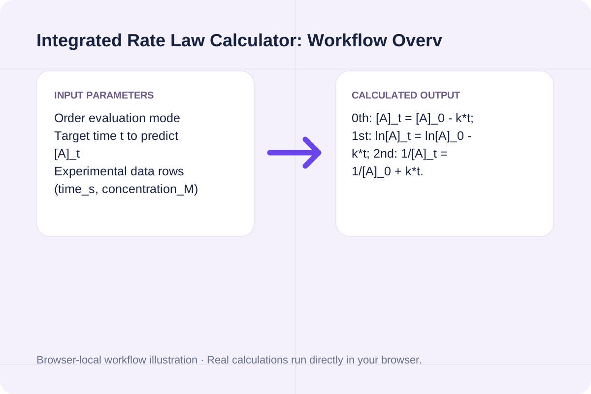
0th: [A]_t = [A]_0 - k*t; 1st: ln[A]_t = ln[A]_0 - k*t; 2nd: 1/[A]_t = 1/[A]_0 + k*t.
Performs ordinary least-squares regression on [A] vs. t, ln[A] vs. t, and 1/[A] vs. t simultaneously, reporting R², residual RMSE in concentration units, fitted [A]_0, rate constant k with exact units, and half-life t_{1/2}.
Reference equations, linear plots, slope meanings, rate constant units, and half-life formulas for single-reactant kinetics (`A -> Products`).
| Reaction Order | Differential Rate Law | Integrated Linear Form | Linear Plot (y vs. x) | Slope & Units of k | Half-Life (t₁/₂) |
|---|---|---|---|---|---|
| Zero Order (`n = 0`) | `Rate = k` | `[A]_t = -k*t + [A]_0` | `[A]` vs. `t` | `Slope = -k` (`M·s⁻¹`) | `[A]_0 / (2k)` |
| First Order (`n = 1`) | `Rate = k[A]` | `ln[A]_t = -k*t + ln[A]_0` | `ln[A]` vs. `t` | `Slope = -k` (`s⁻¹`) | `ln(2) / k ≈ 0.693 / k` |
| Second Order (`n = 2`) | `Rate = k[A]²` | `1/[A]_t = k*t + 1/[A]_0` | `1/[A]` vs. `t` | `Slope = +k` (`M⁻¹·s⁻¹`) | `1 / (k*[A]_0)` |
Enter the values for your scenario, verify the units, and run the calculation.
Start by entering the required fields in the Integrated Rate Law Calculator form above.
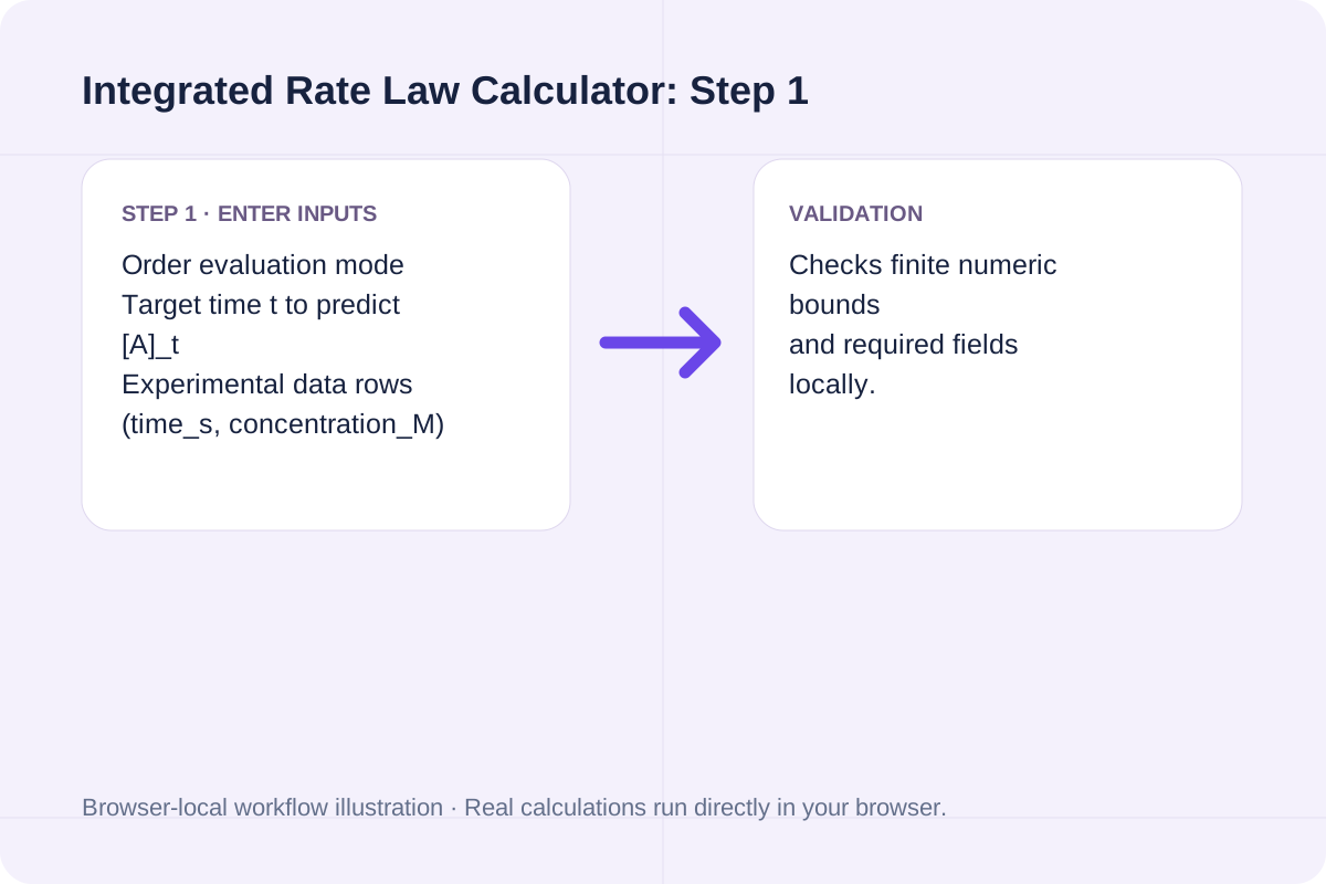
Match each value to the unit or format shown next to the input box before running the calculation.
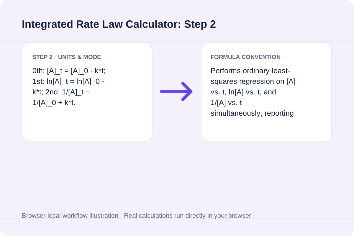
Select Fit Integrated Rate Laws, inspect the primary metric and breakdown cards, then use Copy result or Download result.txt.
Compare baseline and alternative runs for Integrated Rate Law Calculator before exporting the result.
Determine reaction order (0th, 1st, or 2nd) from time-concentration data by linearizing [A], ln[A], and 1/[A] vs. time t, comparing R² and RMSE, and calculating rate constant k and half-life.
0th: [A]_t = [A]_0 - k*t; 1st: ln[A]_t = ln[A]_0 - k*t; 2nd: 1/[A]_t = 1/[A]_0 + k*t.
Performs ordinary least-squares regression on [A] vs. t, ln[A] vs. t, and 1/[A] vs. t simultaneously, reporting R², residual RMSE in concentration units, fitted [A]_0, rate constant k with exact units, and half-life t_{1/2}.
Review the calculated output alongside your entered parameters and unit conventions.
Performs ordinary least-squares regression on [A] vs. t, ln[A] vs. t, and 1/[A] vs. t simultaneously, reporting R², residual RMSE in concentration units, fitted [A]_0, rate constant k with exact units, and half-life t_{1/2}.
Check these three conditions before reporting kinetic parameters.
0th: [A]_t = [A]_0 - k*t; 1st: ln[A]_t = ln[A]_0 - k*t; 2nd: 1/[A]_t = 1/[A]_0 + k*t. Performs ordinary least-squares regression on [A] vs. t, ln[A] vs. t, and 1/[A] vs. t simultaneously, reporting R², residual RMSE in concentration units, fitted [A]_0, rate constant k with exact units, and half-life t_{1/2}.
Calculate average chemical reaction rate, reactant consumption rate, apparent rate constant k, and half-life from initial and final molarity and Δt.
Open tool
Analyze warehouse fulfillment performance from order line data: compute unit fill rate, line fill rate, order fill rate, and backorder recovery with explicit gross vs. net denominators.
Open tool
Calculate bottleneck cycle time, Takt time margin, hourly and shift throughput, line balance efficiency, flow efficiency, and Little's Law WIP from workstation times.
Open toolChoose another tool for your next calculation, conversion, or text task.

Calculate how long it takes to mow any lawn size by deck width, mowing speed, pass overlap, and turn/obstacle field efficiency.
Open tool
Calculate CNC milling and turning Metal Removal Rate (MRR in cm³/min and in³/min), estimated spindle power (kW / HP), and chip load.
Open tool
Calculate hiking time from trail distance, elevation gain, elevation loss, base flat pace, and terrain difficulty using Naismith's Rule, Langmuir descent adjustments, and Tobler's function.
Open tool
Calculate room reverberation time (RT60) using Sabine (0.161 V / A) and Norris-Eyring formulas from room volume and surface absorption coefficients.
Open toolAnswers about using Integrated Rate Law Calculator and understanding its results.
Plot your experimental time-concentration data in three linearized forms: [A] vs. t (zero-order), ln[A] vs. t (first-order), and 1/[A] vs. t (second-order). Whichever transformation yields a straight line with the highest coefficient of determination (R² closest to 1.0000) and random residuals identifies the reaction order.
For a zero-order reaction, k has units of M·s⁻¹ (mol·L⁻¹·s⁻¹). For a first-order reaction, k has units of s⁻¹. For a second-order reaction, k has units of M⁻¹·s⁻¹ (L·mol⁻¹·s⁻¹).
In a first-order reaction, t_{1/2} = ln(2) / k ≈ 0.6931 / k. Because concentration decays exponentially, taking 50% of any starting concentration always requires the exact same time interval. By contrast, zero-order half-life (t_{1/2} = [A]_0 / 2k) decreases as the reaction proceeds, and second-order half-life (t_{1/2} = 1 / (k·[A]_0)) doubles with each successive half-life.
No. Because first-order linearization requires ln[A] and second-order linearization requires 1/[A], every experimental concentration point must be strictly positive ([A] > 0).
Choose another tool for your next calculation, conversion, or text task.